True14 Dimensionality Reduction
14.1 PCA
Examples
We next consider an image approximation (or compression) example where matrix basis are used. Consider the following image:

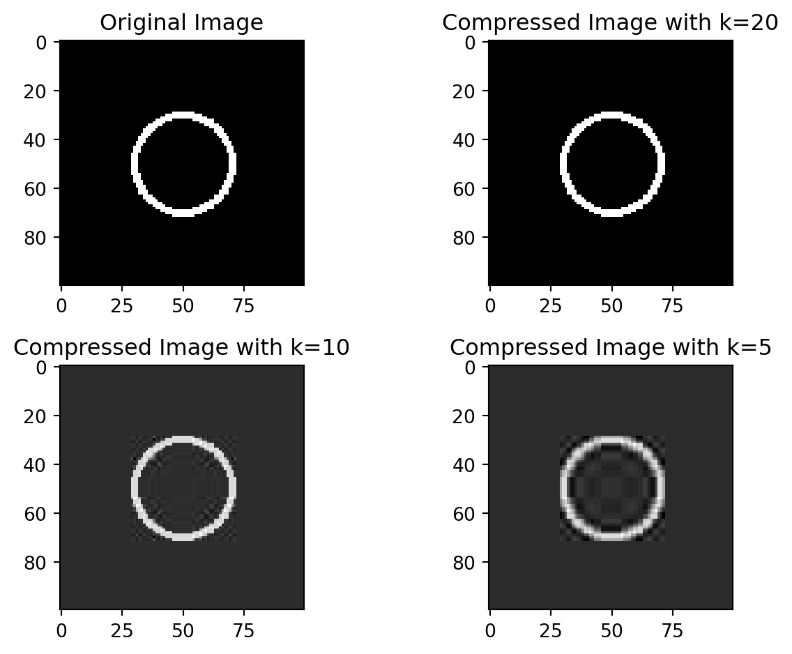
Figure 14.1 shows an image of a circle, which is \(100 \times 100\) in size. While the image is in 2D, the pixel space is \(\mathcal{R}^{100\times 100}\), which needs \(100\times 100=10000\) basis matrices!
However, looking at the image, we can see that most of the image is empty (black pixels) and the circle can be represented with much smaller number of basis functions. Thus, by inspection, we can infer that the image can be represented in a lower dimensional space. We can apply singular value decomposition to determine lower dimensional (or reduced order) representation of the image. This is also known as image compression.
The following Python code demonstrates it.
import numpy as np
import matplotlib.pyplot as plt
from scipy.linalg import svd
from PIL import Image

# Load the image into a numpy array.
img = Image.open('images/circle.png')

# Perform SVD
U, Sigma, Vt = svd(img)

markerline, stemline, baseline = plt.stem(range(len(Sigma)),Sigma)
plt.setp(markerline, markersize = 3)
plt.title("Singular values of the image matrix.")
plt.xlabel("Index k.")
plt.ylabel("Singular Value")
Text(0, 0.5, 'Singular Value')
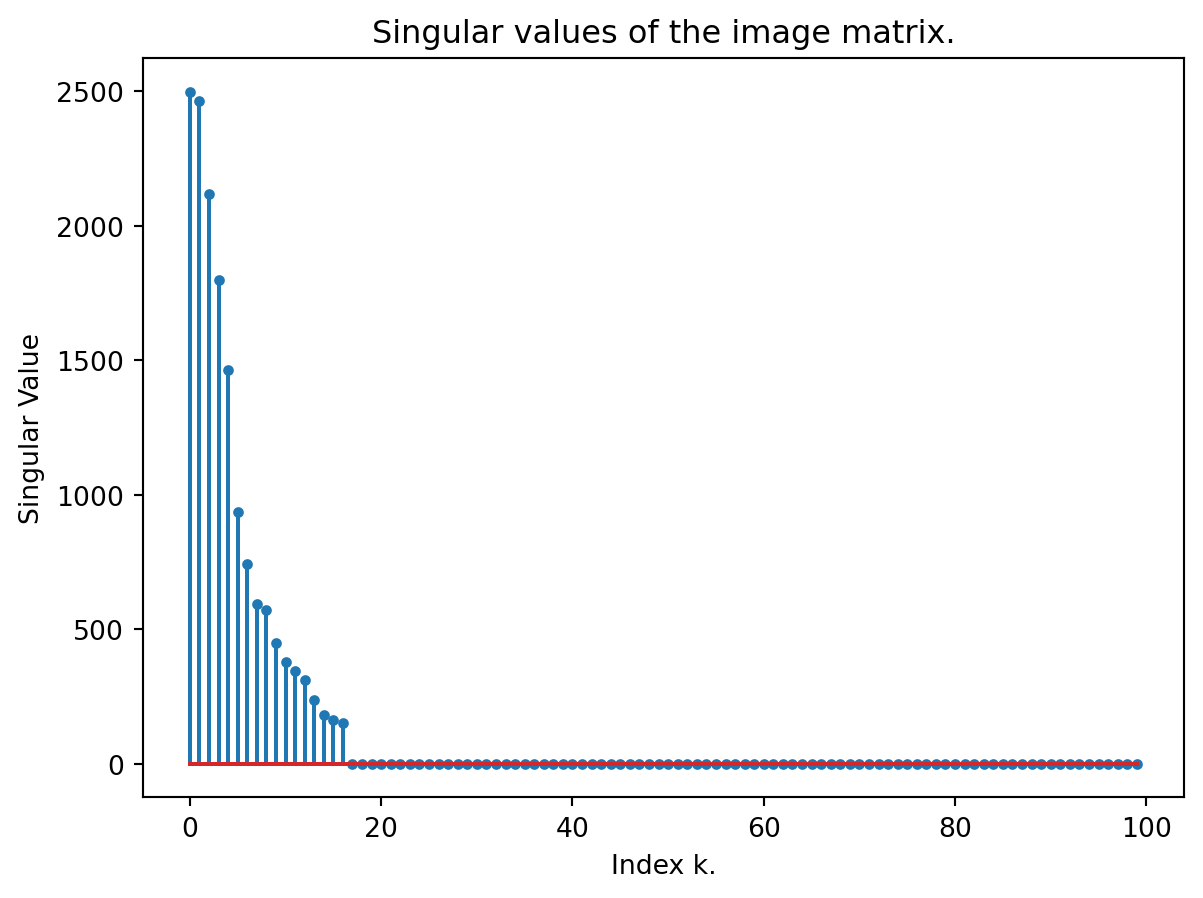
Figure 14.2 shows the singular values of the image matrix. We observe that most of the singular values are zero, indicating the image can be represented in a much lower dimensional space. The next Python code shows how it can be done.
def compress_image(U,Vt,Sigma,k):
  U_k = U[:, :k]
  Sigma_k = np.diag(Sigma[:k])
  Vt_k = Vt[:k, :]
  A_k = np.dot(U_k, np.dot(Sigma_k, Vt_k))
  print(U_k.shape)
  return A_k

img1 = compress_image(U,Vt,Sigma,20)
img2 = compress_image(U,Vt,Sigma,10)
img3 = compress_image(U,Vt,Sigma,5)


# Plot the original and the compressed image
plt.figure()
plt.subplot(2, 2, 1)
plt.imshow(img, cmap='gray')
plt.title('Original Image')

plt.subplot(2, 2, 2)
plt.imshow(img1, cmap='gray')
plt.title('Compressed Image with k=20')

plt.subplot(2, 2, 3)
plt.imshow(img2, cmap='gray')
plt.title('Compressed Image with k=10')

plt.subplot(2, 2, 4)
plt.imshow(img3, cmap='gray')
plt.title('Compressed Image with k=5')

plt.tight_layout()
plt.show()
(100, 20)
(100, 10)
(100, 5)